FaIR-Weather Feedbacks

Permafrost, Methane, and Dieback, Oh My — Implications of Adding New Feedbacks to Simple Climate Models

Feedbacks are central to climate change. However, they are often misunderstood, and no climate model includes all possible feedbacks. Here I discuss the basic concepts behind climate feedbacks, and then show results based on incorporating some of the under-included feedbacks as post-processing add-ons to the reduced complexity FaIR model.

What is a Feedback?

A feedback is what occurs when some process has an effect on itself. A very common example is microphone feedbacks: the sound going into the microphone comes out of the speaker, which feeds back into the microphone, and so on until the whole setup makes a horrible racket.

Note that the microphone example is an example of runaway feedback. Importantly, the Earth is not at risk of runaway feedback due to human emissions of GHGs.

Climate lingo characterizes feedbacks as “positive” or “negative.” Positive feedbacks are bad and negative feedbacks are good… which is confusing, so there is a movement to use terms like “amplifying” and “stabilizing” instead, and I will use those here (for another description of climate feedbacks, see UCAR Center for Science Education, though they use “reinforcing” and “balancing”).

The classic example of an amplifying feedback in climate change is the water vapor feedback. A warmer climate causes more evaporation of water from the oceans. Water vapor is a greenhouse gas, so more water vapor in the atmosphere leads to a warmer climate. Which leads to more evaporation, which… wait, didn’t I say that runaway feedbacks weren’t a thing?

Well, they aren’t. A key demonstration is the following infinite sum:

1 + ½ + ¼ + ⅛ + … = 2

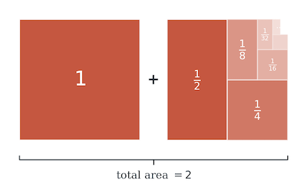
Figure 1 · One unit of warming (left), plus a feedback that adds half as much warming each round and then half of that, and so on (right), sums to just twice the original — amplifying, but not runaway.

So if one unit of warming adds enough water vapor to create half as much warming as the original, then the total effect on the system would be to double the original warming. Not runaway!

So what is the total feedback in the earth system? The standard metric is the climate sensitivity, which is a measure of the warming caused by a doubling of carbon dioxide. The IPCC best estimate for climate sensitivity is 3 °C, with a likely range of 2.5 to 4 °C. Now, the initial warming before feedbacks from a doubling of CO₂ is about 1.2 °C, so the best estimate of the net amplifying feedback is 3 over 1.2, or about a factor of 2.5.¹

This feedback is the result of the sum of a number of key processes, the biggest of which are:

• Planck feedback: the increase in heat loss from the Earth system with any increase in temperature is the key reason that the system does not go to runaway. This is the most important stabilizing feedback. Figure 2 shows it as strongly stabilizing and very certain.

• Water vapor: The increase in water vapor is the biggest and best understood of the amplifying feedbacks (dating back at least to Svante Arrhenius in 1896. The lapse rate is a reference to the cooling rate of the atmosphere with increases in altitude.² Figure 2 shows this as strongly amplifying and very certain.

• Clouds: Clouds are the most uncertain element of the feedback system. Clouds are complicated. Clouds at night warm the surface, clouds in the day cool the surface. High clouds and low clouds have different net effects. Cloud formation is controlled by small scale processes which can’t be simulated in the big GCMs. So while the IPCC best estimates are that clouds are an amplifying feedback, the sign of the feedback is not certain.

• Surface albedo: Ice reflects the sun, cooling the surface. As ice melts and reveals darker ground, this is another amplifying feedback, though smaller than the others.

The IPCC summarized both the best estimates of each of the feedbacks (“AR6”), as well as how they are represented in the prior (CMIP5) and most recent (CMIP6) set of global climate models.

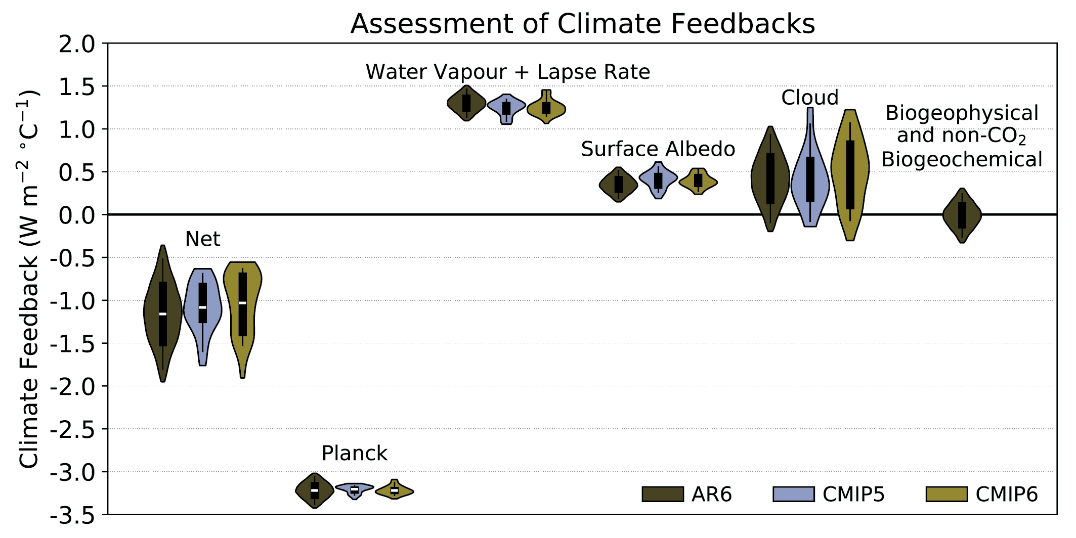
Figure 2 · Global-mean climate feedbacks from abrupt-4×CO₂ runs of 29 CMIP5 (light blue) and 49 CMIP6 (orange) models, against the values assessed in AR6 (red). Reproduced from IPCC AR6 WG1 Figure 7.10.

See also Ripple et al. 2023, where a total of 40 possible feedbacks are discussed. In addition to the key feedbacks discussed above, Ripple et al. discuss second order physical feedbacks like the submergence of coastal lands due to sea level rise decreasing albedo (amplifying) or changes in windblown dust (unclear net effect). Ripple et al. also discuss biological feedback loops like drying and burning peatlands, expanding wetlands, forest dieback, greening of the Arctic (all amplifying) or greening of the Sahara (amplifying through albedo changes, but stabilizing through carbon uptake).

There are a number of flavors of “climate sensitivity”. The “equilibrium” climate sensitivity is the most common – the response of the climate system to a doubling of carbon dioxide, after the system is allowed to relax to equilibrium. There is also the “transient” climate sensitivity: the response of the climate to an increase in carbon dioxide concentrations of 1% per year at the point at which the carbon dioxide doubles (it is always lower than the equilibrium version). The “earth system sensitivity” includes longer term earth system processes like ice sheet retreat, and is higher than the equilibrium version (see Wong et al. 2021). However, all these definitions are based on a doubling of carbon dioxide concentrations, so by definition they don’t include carbon cycle feedbacks. For that, we need the “TCRE” – transient climate response to cumulative carbon emissions (see Steinert and Sanderson, 2025). Because it is based on emissions, not concentrations, it becomes larger when additional carbon cycle effects are included unlike the previous metrics.

With that intro out of the way… time to move on to how feedbacks work in FaIR!

Feedbacks in Reduced Complexity Models

When we discuss climate sensitivity in the big climate models, it is an emergent property that arises out of the physics built into the model (How does water vapor pressure change with temperature? How does air circulate? How are clouds parameterized? Etc.). This means that every big climate model has its own climate sensitivity. In addition to climate models, the IPCC’s best estimates of climate sensitivity are also informed by historical responses to changes in forcing (both over the past century through instrumental records, and over thousands to millions of years through paleoclimate records) as well as their theoretical understanding of the climate system.

One of the key tools used for figuring out what climate sensitivities are consistent with the observational record, as well as for probabilistic projections of future climate change, are the probabilistic models such as FaIR (e.g., Leach et al. 2021). FaIR has 35 key adjustable parameters that together define its climate response, such as ocean heat capacity and rate of heat transfer, forcing for various gases, carbon cycle parameters, and aerosol and aerosol-cloud radiative parameters. Given our understanding of historical patterns of solar intensity, volcanoes, and greenhouse gas concentrations, there can be multiple combinations of these parameters that are consistent with historical temperature observations. For example, if the climate sensitivity is on the high end, then we would also expect the rate of ocean heat uptake or the cooling from aerosols to also be at the high end, otherwise we would have seen more warming (and vice versa).

FaIR also uses future GCM data in its calibration process because there are certain climate responses that we might not have seen in the historical record because the external forcings haven’t been high enough yet, but which are robustly seen across climate models in the future. In this way, a very simple global model implicitly includes a lot of complex processes in its projections. But… if there is a process that hasn’t been observed historically, and isn’t included in the models, then it won’t be included in FaIR unless it is intentionally added.

And that sets up the next section, where I show some preliminary results addressing some of these additional processes.

Adding New Feedbacks to FaIR

I have chosen five processes to focus on that I think are likely underrepresented in FaIR: permafrost thaw³, abrupt permafrost thaw, Amazon forest dieback, wetland methane feedback responses, and the interactions between methane-derived ozone and the carbon cycle. I discuss each in turn, and then the net effects of all five together.

Permafrost thaw (gradual and abrupt)

Thawing permafrost releases both carbon dioxide and methane into the atmosphere, potentially an important amplifying feedback. Most of the models involved in the FaIR calibration did not have explicit permafrost modules. On the other hand, FaIR’s calibration of its historical carbon cycle parameters will have adjusted to the existence of some permafrost emissions.

Woodard et al. 2021 developed an elegant permafrost module for inclusion in the reduced complexity model Hector, but it was straightforward to port this module over to use as a post-processing element for FaIR. Because of the historical calibration issue, I chose to also add an “anti-permafrost” module that is the negative inverse of the permafrost module historical, and then this negative contribution continues in a way that it would exactly cancel any future permafrost emissions from a constant temperature future.

A recent paper by Steinert et al. (2026) also looked at the permafrost amplifying feedback, focusing on how and whether that feedback might lead to triggering certain tipping points that would not have otherwise happened. They used the permafrost response model PerCX. Like me, they used FaIR and did not recalibrate it with the new addition, but as far as I can tell, they did not create an “anti-permafrost” adjustment factor. PerCX has better consistency with AR6 and better uncertainty coverage, but Woodard has a better match to the observed methane fraction of permafrost thaw outgassing and better mechanistic interpretability.

Neither PerCX nor Woodard has an abrupt thaw mechanism, so I also drew on Turetsky et al. (2020) to craft an additional add-on for abrupt thaw.

Amazon dieback

One of the tipping points of concern in the Earth system is that the Amazon forest exists in part because it exists – the rain falling on the Andes feeds the Amazon forest, where it is transpired back into the atmosphere and falls out again in a happy hydrologic cycle. The problem is that with climate change and higher temperatures, in addition to direct human deforestation, we might lose enough of the Amazon forest that the happy hydrologic cycle breaks down and the Amazon shifts into a savannah state. This would have horrible ecological consequences, but for the purposes of this analysis, we just consider how the carbon released by this conversion would be an additional amplifying feedback. We use a module developed by Dietz et al., which has already been used by other researchers, as a supplement to the FaIR model.

Methane-derived ozone and the carbon cycle

The recognition that controlling methane is potentially a good lever not only for reducing climate change but also for reducing air pollution goes back decades – at least to Fiore et al. (2002), though Jason West and Nadine Unger also contributed some key early work in this area. Recognizing this, I have been trying to get the mortality impacts of methane-derived ozone into the social cost of methane since 2017, with updated work in 2023 designed to be consistent with an update in the approach to estimating the social cost of GHGs.

But I’m not talking about mortality in this substack, I’m talking about climate feedbacks. Well, ozone is not only bad for people, it is also bad for plants. My work on the ozone/ecosystem linkage dates back to 2005. If it is bad for natural plants, it is also bad for agriculture – see my 2023 paper.

In any case, if plants are damaged by ozone produced by methane, that leads to reduced carbon sequestration, which leads to increased carbon dioxide concentrations – an amplifying feedback! For this work, I relied primarily on the relationship between ozone and carbon cycle impacts from Unger et al. 2020, and the relationship between methane and ozone is based on the approach we used in McDuffie et al..

Like for permafrost, it is also important to add a negative factor to cancel out the effects historically. The addition of this factor means that the net effect of adding this interaction in terms of future baseline scenarios is small – however, when considering marginal emission changes of methane alone the effect can be more substantial.

This is not novel work – Collins et al. did a similar calculation in 2010 – but it is still not incorporated into mainstream modeling and therefore worth revisiting and doing the background work to make it useable by reduced complexity modelers.

Wetland methane emissions

The last of the feedbacks that I considered for this post are methane emissions from global wetlands, which are expected to increase due to increased precipitation and inundation in many regions. Here I rely on Ury et al. (2025).

Model Results

So what happens once these feedbacks are bolted onto FaIR? We can start by looking at the increase in radiative forcing in the year 2100. The first change to note is the increase in the median forcing, from 5.2 W/m² to 5.6 W/m². In the old RCP framework, this tips the scenario that is nearest to the median from RCP4.5 to RCP6.0. At the high end, the probability of exceeding 8.5 W/m² has gone from 0.9% to 3% – making RCP8.5 less implausible than before. This is also a lesson in overinterpreting the tails of the distribution: it is easy to go from less than 1% (perhaps more implausible than is worth including in a group of scenarios) to 3% (possibly worth including in worst case scenario planning) very easily (note that the wiggles in the forcing are due to the solar cycle).

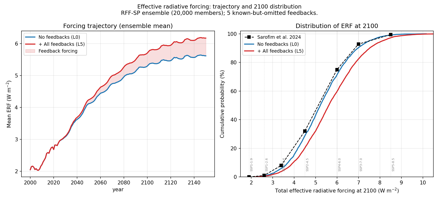
Figure 3 · Radiative forcing in 2100 across the RFF-SP ensemble, with and without the five feedbacks. Left: mean forcing over time, shaded band = the feedback contribution. Right: the full 2100 distribution as a cumulative curve, with SSP-RCP levels and the Sarofim et al. 2024 baseline marked.

We can also look at changes in baseline temperature and sea level rise projected across the full RFF-SP emissions ensemble. Feedbacks shift the whole distribution warmer and higher.

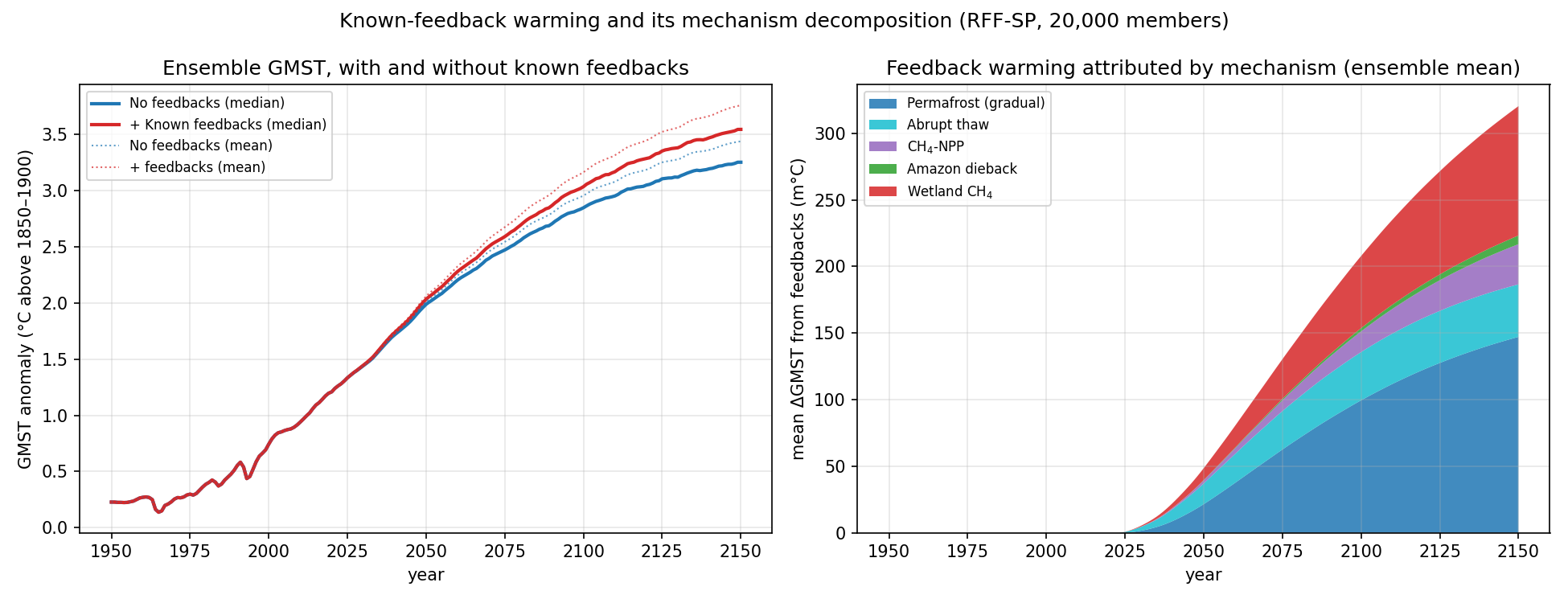
Figure 4 · Baseline warming across the ensemble. Left: median (and mean) global temperature with and without the feedbacks. Right: the added warming split by mechanism — gradual permafrost dominates, then wetland methane and abrupt thaw.

Adding these feedbacks adds about 0.2 °C to the median expected warming in 2100… and more than 0.4 °C to the 95% warming percentile. The largest contributor is gradual permafrost thaw, followed by wetland methane, abrupt permafrost thaw, the methane-derived ozone carbon cycle impacts, and finally Amazon dieback. Because of the long right tail, the mean is higher than the median. Amazon dieback is only triggered at higher temperatures, so contributes more to the mean than the median.

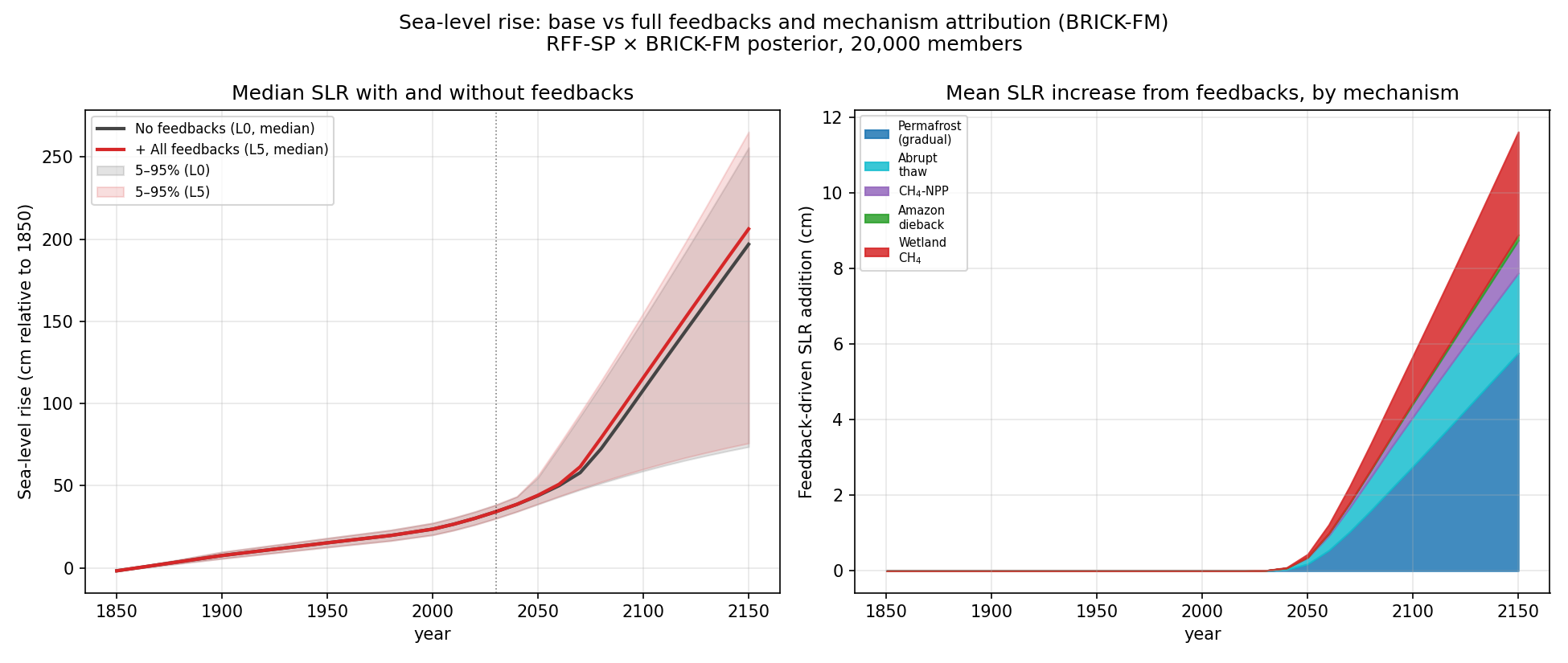
Figure 5 · Baseline sea level rise (BRICK-FM). Left: median rise with and without the feedbacks, with 5–95% ranges. Right: the feedback-driven addition split by mechanism.

Sea level rise tells a similar story. On the BRICK-FM posterior, the feedbacks raise the median projected sea level rise in 2100 by roughly 8 cm, an increase of about 7% over the no-feedback median. The absolute addition is smaller in the upper tail (+4 cm at the 95th percentile) than at the median. One caveat, on the levels rather than the shift: these come from a single sea-level model, and BRICK-FM has a larger Antarctic contribution to end of century sea level rise than some other models.

While the baseline shifts are interesting, even larger shifts occur when looking at the impact of a marginal tonne of emissions. And something I’ve been interested in for a long time (see Sarofim & Giordano 2018 for my best paper on the subject to date) is the relative impacts of CO₂ and methane.

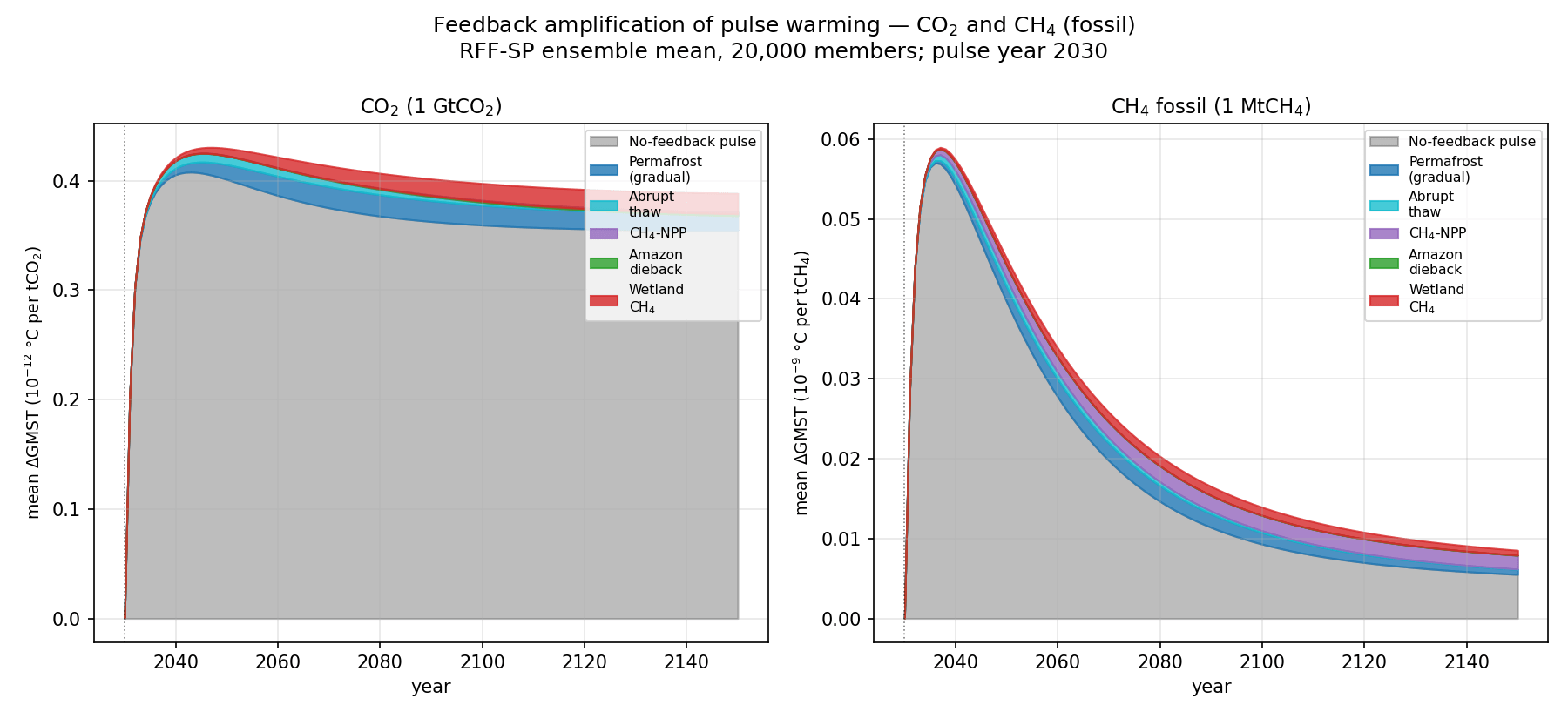
Figure 6 · Warming per GtCO₂ from a CO₂ pulse (left) and per MtCH₄ from a fossil-methane pulse (right), released in 2030. Grey is the no-feedback response; colored bands stack the extra warming from each feedback.

The feedbacks have a greater relative effect on a pulse of methane emissions than on a pulse of CO₂ emissions. This is partially because the CH₄–O₃–NPP effect is specific to CH₄, but also because all the carbon cycle effects add long-lived CO₂ to the earth system, which persists long after the methane has oxidized in the atmosphere.

The cleanest way to see the asymmetry is to put methane and CO₂ on a common per-tonne footing. The table below compares several methane-to-CO₂ equivalency metrics with no feedbacks and with all five feedback layers (the four processes above, counting permafrost’s gradual and abrupt thaw separately). Note that the Pseudo-GWP-100 is nearly double the traditional GWP-100 because of the increasing background CO₂ concentration in these calculations, versus the constant background concentration in the traditional GWP calculation.

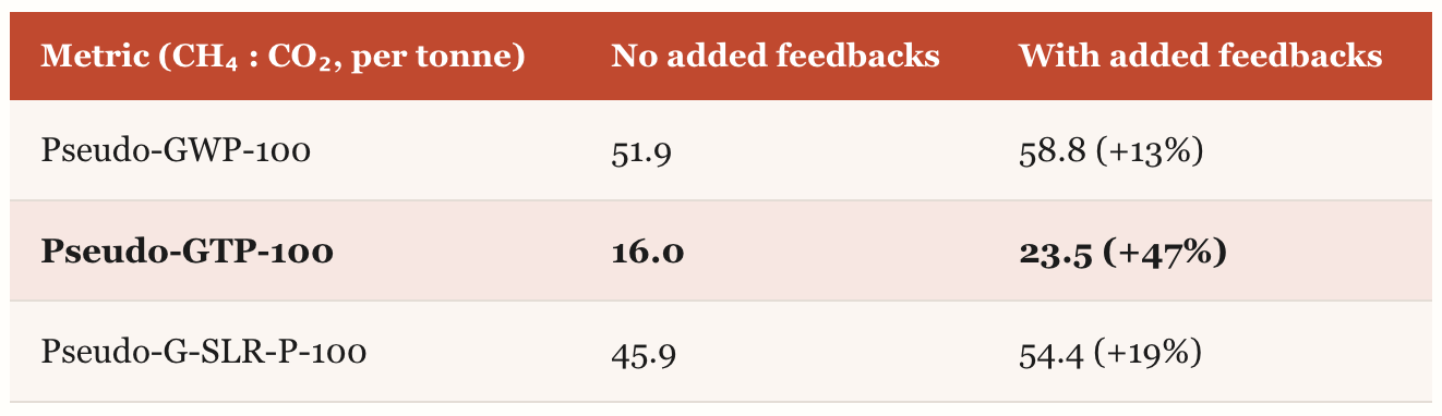
Methane-to-CO₂ equivalency, per tonne, ensemble median, pulse year 2030. “No added feedbacks” is native FaIR (L0); “+ feedbacks” shows the effects of the additional feedbacks discussed here (L5). Biogenic methane (e.g. cow burps) adds no new carbon to the atmosphere; fossil, old-carbon methane (e.g. permafrost) does. GWP / GTP / G-SLR-P = 100-year global warming / temperature / sea-level-rise potentials. “Pseudo” because each is computed on the evolving RFF-SP background rather than on a constant concentration background: this contributes to higher ratios than the traditional GWP. Biogenic methane, with no oxidation CO₂ tail, runs about 2 lower than fossil at the feedback level – for example a pseudo-GWP-100 of 56.4 versus 58.8.

The GWP is the integrated radiative forcing over the century, the GTP is the temperature at the end of the century: the former is roughly the average effect on climate over that period, and the latter is the effect only at the end. This is why the GTP-100 for methane is substantially lower than the GWP-100 for methane. Adding long-lived carbon through carbon cycle effects therefore has a relatively larger effect on the GTP than on the GWP (though a very similar absolute change). One caveat: each of these feedbacks was calculated based on the original pulse: however, there would be an additional amplifying effect if I allowed the feedbacks to interact with each other.

Methane, per ton, has more than twice the carbon of CO₂, which is why the GWP and GTP for biogenic methane are about 2 less than for fossil methane.

It is worth flagging that the land carbon sink keeps showing up as the common thread. A recent paper by Tang et al. showed that inclusion of nitrogen limitation meaningfully weakened the terrestrial carbon sink by limiting the benefits of carbon fertilization. I know that nitrogen limitation in terrestrial ecosystem models was something that the Terrestrial Ecosystem Model I used in grad school did better than many other models at the time – I wonder if the Tang et al. paper also considered the stabilizing feedback that increased temperatures lead to more soil nitrogen release as in Melillo et al. 2002.

The five feedback layers are packaged as a standalone Python module, fair-feedbacks, with a minimal FaIR-coupling example and unit tests, so anyone can reproduce or build on the analysis.

Conclusions

None of the five feedbacks I have added here is news to the scientific community – permafrost thaw (regular and abrupt), Amazon dieback, the methane-ozone-carbon link, and wetland methane are all well documented. What is missing is their inclusion in the reduced-complexity models that increasingly underpin probabilistic projections and the social cost of greenhouse gases. Bolting them on as post-processing add-ons is a stopgap, but allows for quantification of the magnitude of this effect. The effect on baseline temperature and sea level is real if bounded: it raises median warming in 2100 by about two tenths of a degree, and more than four tenths at the upper end of the range, with an 8 cm increase in sea level rise. The effect on how we value methane relative to CO₂ is larger because it adds a long carbon tail to short-term effects of the methane pulse. As more of these carbon-cycle feedbacks are characterized well enough to emulate, the case for building them into the standard toolkit – rather than bolting them on after the fact – only gets stronger.

1. The alternate way of measuring feedback is the 1−f approach, where a feedback of 1 or greater is runaway. This is relevant to Bayesian approaches of estimating total system feedbacks: some studies use a prior over climate sensitivity (equal probability between 0 and 10), whereas others use a prior over the feedback factor (equal probability between 0 and 1), yielding somewhat different results – see Roe and Baker 2007.

2. Up to the tropopause. An alternate way of thinking about climate feedbacks is that they adjust the height of the tropopause, which is defined by the height at which radiative loss is in balance. The higher the tropopause, the higher the surface temperature.

3. Permafrost experts can get very antsy if you talk about permafrost “melt.” As they point out, if you take a chicken out of the freezer it thaws, it doesn’t melt. Permafrost is frozen soil, so similarly, it thaws, it does not melt.